Everything you need to know about managing multiple versions of a graph atomically

A graph is a data structure that consists of nodes and edges joining two nodes. The graph data structure has many use cases.

Graph storage and traversal are simplified by graph databases such as AWS Neptune or Neo4j. A graph database allows storing a graph in the form of nodes and edges. Each node and edge are identified by a unique identifier. Additionally, one can attach properties and labels to nodes and edges.

An example of a graph representing a social network can be seen below:

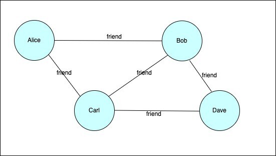
This graph consists of four nodes (Alice, Bob, Carl, and Dave) and five edges representing the relation ‘friend’ between specific pairs of nodes.

There are two common types of graphs: property graphs and RDF graphs. The discussion in this blog applies to property graphs and any graph database that allows attaching labels and properties to nodes and edges, such as AWS Neptune and Neo4j. It also applies to both directed and undirected graphs. We will use a directed graph in AWS Neptune as an example in this blog.
A property graph stored in a graph database can be traversed using different query languages, such as Gremlin and OpenCypher.

In Amazon, we had the use case as described below:
A graph is received as input in the form of a file. The graph needs to be stored in a database, which will then be queried by a user-facing client service.

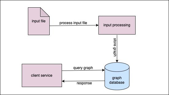
Once the initial graph is stored, a new batch update file is received every week that contains a batch of node / edge updates, that is, additions and removals as compared to the previous file. These updates need to be incorporated into the graph, thus creating subsequent versions of the graph.
The client service must:

• see a consistent view of the graph at all times, which means a new version of the graph should reflect in query results only after the entire update file has been processed.
• be able to query the last ‘N’ versions of the graph.

As an example, consider the following file received initially at week 0:Nodes

Edges

This leads to the following version 0 of the graph:

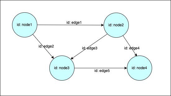
The following update file is received at week 1:
Nodes

Edges

The update includes addition of node5 and removal of node4. edge4 and edge5 connected to node4 are also removed. This leads to the following version 1 of the graph:

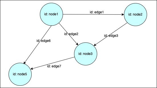
The following update file is received as yet another update at week 2:
Nodes

Edges

The update includes addition of node6 and edge8. This leads to the following version 2 of the graph:

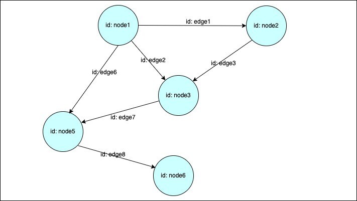
For a client service to always see a consistent version of the graph, the batch of updates in the file needs to be applied atomically, and an external storage is needed to indicate that the new version is available to be queried. External storage refers to any storage outside the graph database, such as a configuration store or client service memory. Let’s call it the version datastore.

A naive approach to achieving this would be to create a new graph altogether when the batch update file is received by following the below steps:

• Copy the existing graph.
• Apply the updates received in the batch update file.
• Update the version datastore to indicate the new graph is ready.

While this approach works, it has the disadvantage of a large storage requirement because common parts of the graph are duplicated multiple times.
In the following section, we will discuss two approaches to achieve atomicity and store multiple versions within the same graph, thus reducing data duplication.

Time-slicing is a standard technique to query graph revision data. At its core, it involves adding ‘created’ and ‘expired’ timestamps to each vertex and/or edge, indicating the time when it became valid and invalid respectively. To query the state of the graph at timestamp ‘t’, the client service then has to use the filter ‘created <= t < expired’.
As an example, consider the graph below:

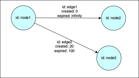
This graph indicates that the relation between node1 and node2 is valid from timestamp 0 up to infinity, and the relation between node1 and node3 is valid from timestamp 20 up to timestamp 100. In practice, these timestamps could be epoch millisecond values, and infinity could be represented by the maximum integer value supported by the system.
To get all outgoing nodes from node1 at timestamp 5, client service can use the following Gremlin query:
g.V().hasId('node1').outE().has('created', lte(5)).has('expired', gt(5)).inV()

However, processing the batch of updates in a file one by one and storing continuous timestamps does not guarantee file-level atomicity. This is because each update would start reflecting in query results as soon as it was applied.

To achieve atomicity, we will use a file-level version number instead of edge/node-level timestamps and use the version datastore to indicate when a version is ready to be queried. The client service can then check the version datastore for versions available for query, and then query the graph for those versions.
Therefore, each edge is augmented with a ‘created’ property that indicates the version number at which the edge was added and an ‘expired’ property that indicates the version number at which the edge became invalid.

For the example that we described in the ‘Use case description’ section, the sequence of events looks as follows:
At week 0, the initial input file is received, and the following graph is stored:

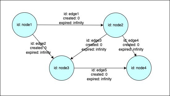
The version datastore is updated to indicate that version 0 is ready, and the client service can query it.

At week 1, the batch update file is received, after which the graph is updated as below:

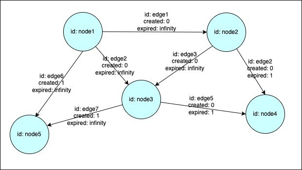
In this version, ‘expired’ property of edge4 and edge5 has been updated to 1, indicating that they expired in version 1. edge6 and edge7 were created with ‘created’ property as 1, indicating that they were added in version 1.
The version datastore is then updated to indicate that version 1 is ready. At this point, the client service can query either version 0 or version 1 by filtering ‘created’ and ‘expired’ properties accordingly. For example,
query for all outgoing nodes from node3 in version 0: g.V().hasId('node3').outE().has('created', lte(0)).has('expired', gt(0)).inV() – returns node4
query for all outgoing nodes from node3 in version 1: g.V().hasId('node3').outE().has('created', lte(1)).has('expired', gt(1)).inV() – returns node5,

This process is repeated every time a new batch update file is received.

In this approach, instead of using ‘created’ and ‘expired’ properties, we use edges to represent the last N versions. Each edge represents a version amongst the last N versions. Let’s assume that the client service needs to be able to query the last three versions.
Instead of connecting nodes by one edge, we will connect them by three edges, each bearing a label that corresponds to a version.

For the sample input files we used in the previous section, the sequence of events is as follows:
At week 0, the initial input file is received, and the following graph is stored:

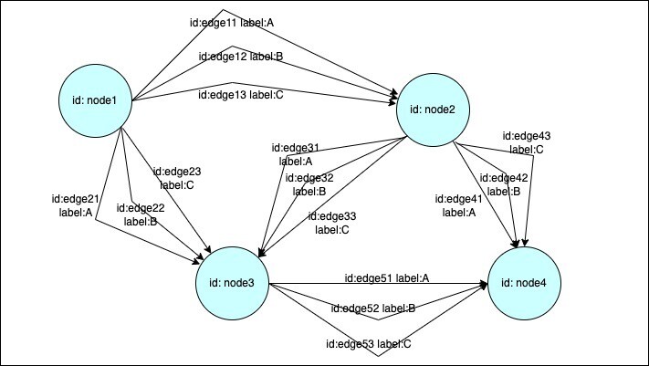
As can be seen above, we have added three edges between pairs of nodes, labelled ‘A’, ‘B’, and ‘C’. These correspond to three consecutive versions.
The version datastore is updated to store the following relation between edge label and version number:

Here, versions -2 and -1 are dummy versions required for bootstrap, and version 0 is the first real version that can be queried by client service. This is indicated by the ‘Status’ column. At this point, the client service can query the version datastore to check that version 0 is ACTIVE, and then query the graph for version 0 using edge label ‘C’.
For example, query to get outgoing nodes from node3: g.V().hasId('node3').outE('C').inV() – returns node4.

At week 1, the first batch update file is received. The collated updates across the last three update files are applied to edges labelled ‘A’. However, initially we have only one update file, for which updates are applied, after which the graph is as below:

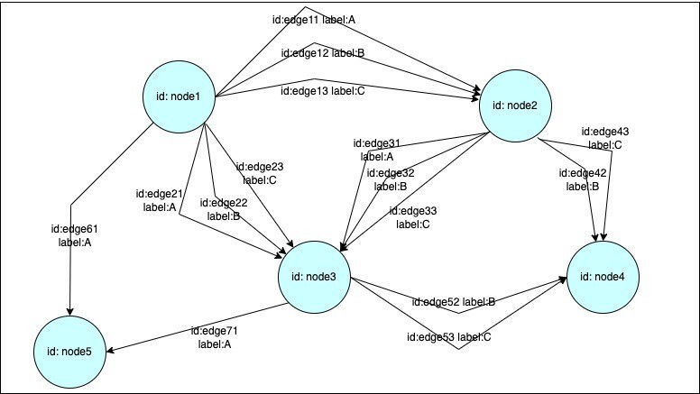
The mapping in version datastore is then updated as below:

This indicates that edges labelled ‘A’ now correspond to version 1. At this stage, client service can query version 0 using edge label ‘C’, and version 1 using edge label ‘A’. For example, query to get outgoing nodes from node3 in version 0: g.V().hasId(‘node3’).outE(‘C’).inV() – returns node4
query to get outgoing nodes from node3 in version 1: g.V().hasId(‘node3’).outE(‘A’).inV() – returns node5

At week 2, the next batch update file is received. The collated updates in the last three files need to be applied to edges labelled ‘B’. However, at this stage, we have only two update files for which updates are applied, after which the graph is as below:

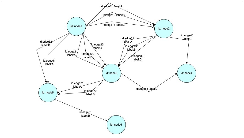
The mapping in version datastore is then updated as below:

This indicates that edges labelled ‘B’ now correspond to version 2. At this stage, client service can query version 0 using edge label ‘C’, version 1 using edge label ‘A’, and version 2 using label ‘B’. For example, query to get outgoing nodes from node5 in version 2:
g.V().hasId(‘node5’).outE(‘B’).inV() – returns node6

This sequence continues every time a new batch update file is received. When a new update file is received at week 3, the collated updates across the last three batch update files are applied to edges labelled ‘C’, after which the mapping in version datastore is updated as below:

It is worth noting that at this point, node4 is a dangling node, that is, a node with no connected edges. Please refer to the ‘Closing notes’ section in the end for further discussion on dangling nodes.
While both the above described approaches work, it is important to understand the trade-offs while choosing one of them. The two major parameters for trade-off here are storage size and query latency. While the exact storage size and query latency will depend on the underlying implementation of the graph database being used, the general analysis should be similar.
We will use AWS Neptune as an example to analyse the trade-offs.

Storage size: AWS Neptune stores data in the form of four-position (quad) elements. The 4 positions of a quad are Subject(S), Predicate(P), Object(O), Graph(G). For an edge to be stored along with a label, the Subject(S) is the ‘from’ vertex, the Predicate(P) is the user-supplied edge label, the Object(O) is the ‘to’ vertex, the Graph(G) is the edge identifier.
For an additional property to be stored for an edge, a quad is used where the Subject(S) is the edge identifier, the Predicate(P) is the property name, Object(O) is the property value, and Graph(G) is null.

Thus, in the first approach in Figure 7, storing ‘edge1’ between ‘node1’ and ‘node2’, along with ‘created’ and ‘expired’ properties will need three quads to be stored as below:

In the second approach in Figure 9, storing ‘edge11’ between ‘node1’ and ‘node2’ along with label ‘A’ will need one quad as below:

This translates to three quads for three edges as below:

It is then apparent that the second approach would require less storage space when the number of versions to be maintained is small, say two or three. The storage space for second approach will be increase as the number of versions to be stored increases, while it will remain constant for the first approach.
Query latency: In the first approach, the query latency will be higher since it needs to query the ‘created’ and ‘expired’ properties of the edges, and filter on those properties. In the second approach, only the edge needs to be queried with the label, leading to lower latency.

It is worth re-iterating that one should benchmark the storage space and query latency for these approaches before deciding on one.

The reader might have observed that so far we have talked about the addition and removal of nodes and edges but not about updates to existing node properties.
Consider the social network example in Figure 1. Assume that along with the nodes representing individuals, we also store properties such as phone number, email address, etc. Some of these properties can change over time.

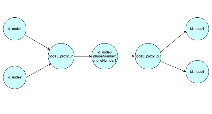
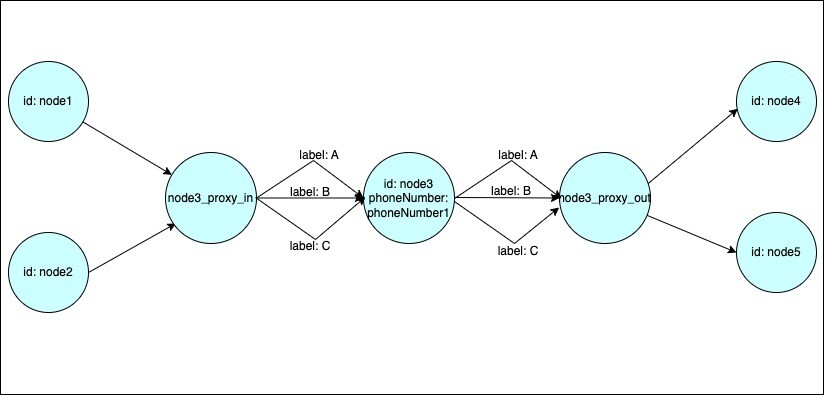
The simplest approach to managing node property updates would be to create a new node and expire the old node. However, this means all edges connected to the node will also have to be copied, which can be a major performance issue if the number of edges is large. To avoid having to copy all edges, we can use proxy nodes. Each node is joined by one edge to a proxy_in node and by another edge to a proxy_out node. All incoming edges to this node now connect to the proxy_in node; and all outgoing edges from this node now connect to the proxy_out node.
As an example, consider the graph below:

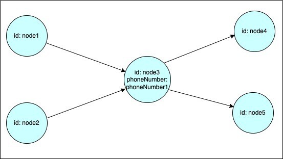
On applying proxy nodes to node3, the graph looks as below:

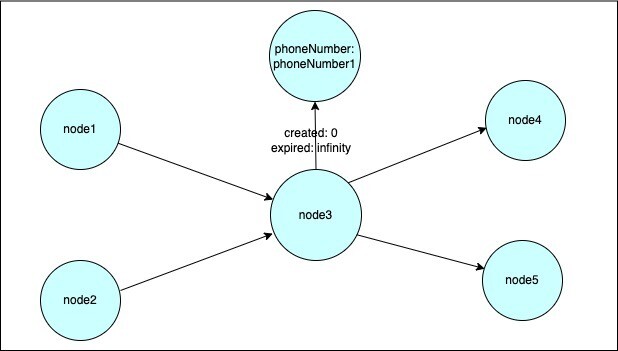
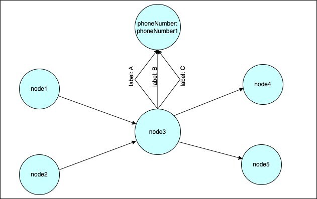
Another approach to manage node property updates is to separate the node from its state, as exemplified below:

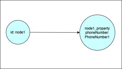
The second approach would require slightly lower storage size and offer slightly lower query latency, since it uses fewer nodes and edges to store the same information. However, both approaches are comparable, and one can choose either depending on how one wants to model the data.

Let us now see how we can use the two approaches discussed in the ‘Solution’ section with proxy nodes to achieve atomicity and multiple versions support for node property updates.

Consider the initial version 0 of graph as below:

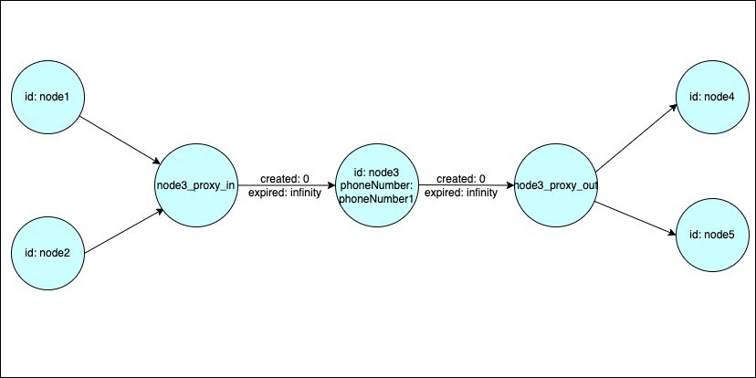
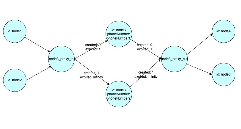
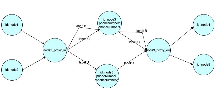
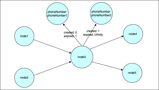
In version 1, the ‘phoneNumber’ property of node3 is updated to ‘phoneNumber2’. The graph is then updated as below:

Using the second approach of using edges as version number, the initial graph is stored as below:

In version1, when the ‘phoneNumber’ property of node3 is updated to ‘phoneNumber2’, the graph is updated as below:

Let us now see how we can use the two approaches discussed in the ‘Solution’ section with separation of node and properties to achieve atomicity and multiple versions for node property updates.
For the graph represented in Figure 12, using the first approach of time-slicing, the initial version of the graph is stored as below:

In version 1, when the ‘phoneNumber’ property of node3 is updated to ‘phoneNumber2’, the graph is updated as below:

For the same graph, following the second approach of using edges as versions, the initial version of the graph is stored as below:

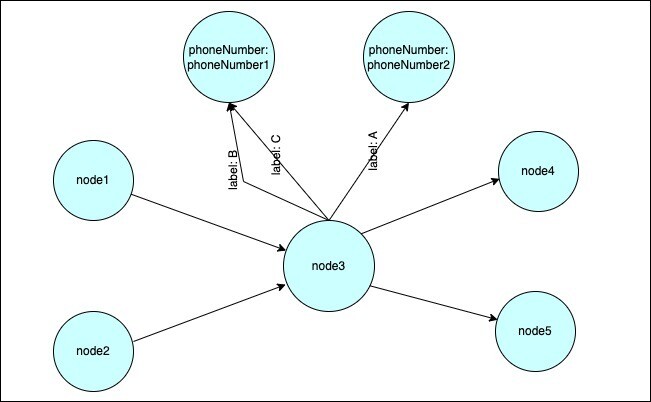
In version 1, when the ‘phoneNumber’ property of node3 is updated to ‘phoneNumber2’, the graph is updated as below:

We will now put together the various techniques we discussed in the previous sections and write down a detailed algorithm following one of the approaches for a sample use case. We will write Gremlin queries for each of the steps.

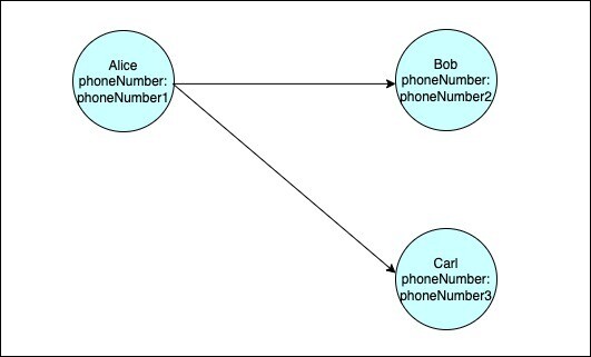
Consider a social network graph where each node represents a person and has an associated property called ‘phoneNumber’. We need to support querying the last three versions and achieve atomicity in version updates.

The following input is received at week 0:
Nodes

Edges

This corresponds to the following graph in version 0:

Following Approach 2 of using edges as versions, and using proxy nodes for node properties, we will create the initial graph as below:

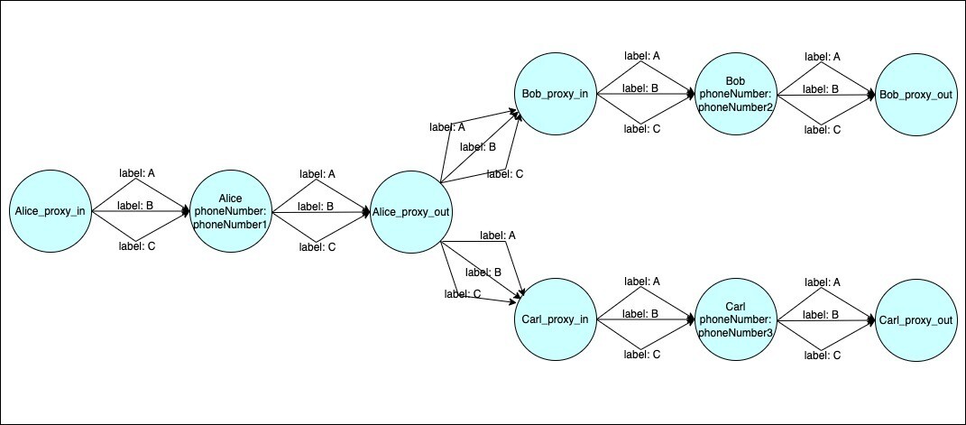
Steps:

• Create ‘Alice’ nodes
  
  • g.addV().property(id, ‘Alice’).property(‘phoneNumber’, ’phoneNumber1’)
  • g.addV().property(id, ‘Alice_proxy_in’)
  • g.addV().property (id, ‘Alice_proxy_out’)
• Add edges labelled ‘A’, ‘B’, and ‘C’ between ‘Alice’ nodes
  
  • g.V('Alice_proxy_in').as('fromV').V('Alice').as('toV').addE('A').from('fromV').to('toV')
  • g.V('Alice').as('fromV').V('Alice_proxy_out').as('toV').addE('A').from('fromV').to('toV')
  • g.V('Alice_proxy_in').as('fromV').V('Alice').as('toV').addE('B').from('fromV').to('toV')
  • g.V('Alice').as('fromV').V('Alice_proxy_out').as('toV').addE('B').from('fromV').to('toV')
  • g.V('Alice_proxy_in').as('fromV').V('Alice').as('toV').addE('C').from('fromV').to('toV')
  • g.V('Alice').as('fromV').V('Alice_proxy_out').as('toV').addE('C').from('fromV').to('toV')
• Repeat the above 2 steps for ‘Bob’ and ‘Carl’ nodes
  
  • g.addV().property(id, 'Bob’).property('phoneNumber', 'phoneNumber2')
  • g.addV().property(id, 'Bob_proxy_in')
  • g.addV().property (id, 'Bob_proxy_out')
  • g.V('Bob_proxy_in').as('fromV').V('Bob').as('toV').addE('A').from('fromV').to('toV')
  • g.V('Bob').as('fromV').V('Bob_proxy_out').as('toV').addE('A').from('fromV').to('toV')
  • g.V('Bob_proxy_in').as('fromV').V('Bob').as('toV').addE('B').from('fromV').to('toV')
  • g.V('Bob').as('fromV').V('Bob_proxy_out').as('toV').addE('B').from('fromV').to('toV')
  • g.V('Bob_proxy_in').as('fromV').V('Bob').as('toV').addE('C').from('fromV').to('toV')
  • g.V('Bob').as('fromV').V('Bob_proxy_out').as('toV').addE('C').from('fromV').to('toV')
  • g.addV().property(id, 'Carl').property('phoneNumber', 'phoneNumber3')
  • g.addV().property(id, 'Carl_proxy_in')
  • g.addV().property (id, 'Carl_proxy_out')
  • g.V('Carl_proxy_in').as('fromV').V('Carl').as('toV').addE('A').from('fromV').to('toV')
  • g.V('Carl').as('fromV').V('Carl_proxy_out').as('toV').addE('A').from('fromV').to('toV')
  • g.V('Carl_proxy_in').as('fromV').V('Carl').as('toV').addE('B').from('fromV').to('toV')
  • g.V('Carl').as('fromV').V('Carl_proxy_out').as('toV').addE('B').from('fromV').to('toV')
  • g.V('Carl_proxy_in').as('fromV').V('Carl').as('toV').addE('C').from('fromV').to('toV')
  • g.V('Carl').as('fromV').V('Carl_proxy_out').as('toV').addE('C').from('fromV').to('toV')
• Create 3 edges from ‘Alice_proxy_out’ to ‘Bob_proxy_in’, labelled ‘A’, ‘B’, and ‘C’
  
  • g.V('Alice_proxy_out').as('fromV').V('Bob_proxy_in').as('toV').addE('A').from('fromV').to('toV')
  • g.V('Alice_proxy_out').as('fromV').V('Bob_proxy_in').as('toV').addE('B').from('fromV').to('toV')
  • g..V('Alice_proxy_out').as('fromV').V('Bob_proxy_in').as('toV').addE('C').from('fromV').to('toV’)
• Create 3 edges from ‘Alice_proxy_out’ to ‘Carl_proxy_in’, labelled ‘A’, ‘B’, and ‘C’.
  
  • g.V('Alice_proxy_out').as('fromV').V('Carl_proxy_in').as('toV').addE('A').from('fromV').to('toV')
  • g.V('Alice_proxy_out').as('fromV').V('Carl_proxy_in').as('toV').addE('B').from('fromV').to('toV')
  • g.V('Alice_proxy_out').as('fromV').V('Carl_proxy_in').as('toV').addE('C').from('fromV').to('toV')
• Update version datastore with the following mapping:

• Client service can then query version 0 using label ‘C’, using the following steps
  
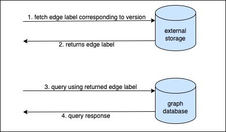
  • Query version datastore to fetch the edge label corresponding to version 0. This will return ‘C’.
  • Query the graph using edge label ‘C’. Sample Gremlin query to get outgoing nodes from ‘Alice’: g.V().hasId('Alice_proxy_out').outE('C').inV().outE('C').inV() – returns ‘Bob’ and ‘Carl’

At week 1, the first batch update file is received:
Nodes

Edges

This corresponds to the following graph in version 1:

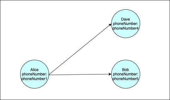
The updates will be applied to ‘A’ labelled edges since it is the next label after the current latest label ‘C’, leading to the following graph:

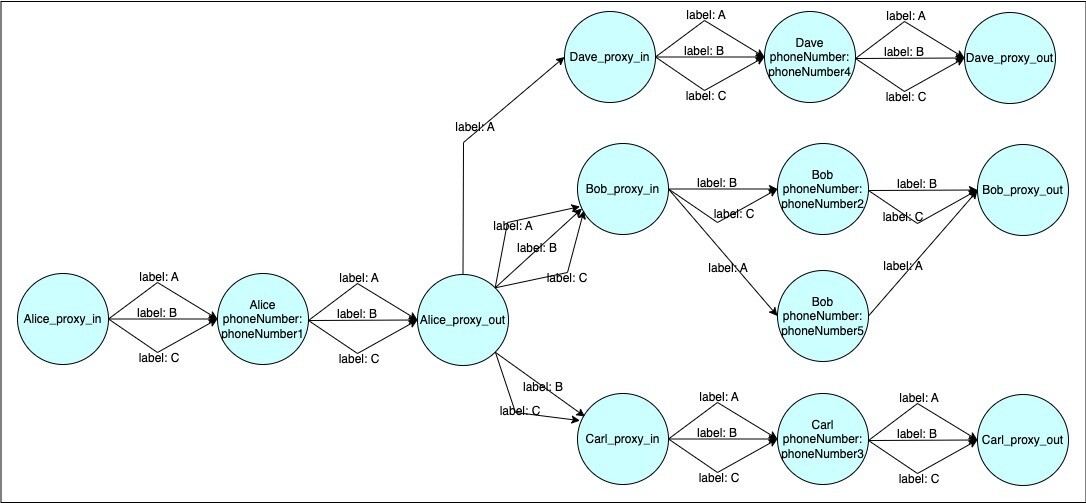
Steps:

• Query the version datastore to fetch the label corresponding to the latest version. Currently, it is ‘C’. The next version will be created with the next label, which is ‘A’.
• Create ‘Dave’ nodes
  
  • g.addV().property(id, 'Dave').property('phoneNumber', 'phoneNumber4')
  • g.addV().property(id, 'Dave_proxy_in')
  • g.addV().property (id, 'Dave_proxy_out')
• Add edges labelled ‘A’, ‘B’, and ‘C’ between ‘Dave’ nodes
  
  • g.V('Dave_proxy_in').as('fromV').V('Dave’).as('toV').addE('A').from('fromV').to('toV')
  • g.V('Dave').as('fromV').V('Dave_proxy_out').as('toV').addE('A').from('fromV').to('toV')
  • g.V('Dave_proxy_in').as('fromV').V('Dave').as('toV').addE('B').from('fromV').to('toV')
  • g.V('Dave').as('fromV').V('Dave_proxy_out').as('toV').addE('B').from('fromV').to('toV')
  • g.V('Dave_proxy_in').as('fromV').V('Dave’).as('toV').addE('C').from('fromV').to('toV')
  • g.V('Dave').as('fromV').V('Dave_proxy_out').as('toV').addE('C').from('fromV').to('toV')
• To remove ‘Carl’ from this version, remove ‘A’ labelled edge connecting ‘Alice_proxy_out’ to ‘Carl_proxy_in’
  
  • g.V().hasId('Alice_proxy_out').outE('A').as('edge').inV().hasId('Carl_proxy_in').select('edge').drop()
• Add ‘A’ labelled edge connecting ‘Alice_proxy_out’ to ‘Dave_proxy_in’
  
  • g.V('Alice_proxy_out').as('fromV').V('Dave_proxy_in').as('toV').addE('A').from('fromV').to('toV')
• To update the phoneNumber property of ‘Bob’, create a new ‘Bob’ node and connect it to corresponding proxy nodes through ‘A’ edges (use a unique identifier such as ‘Bob_<uuid>’)
  
  • g.addV().property(id,'Bob_2').property('phoneNumber', 'phoneNumber5')
  • g.V().hasId('Bob_proxy_in').outE('A').as('edge').inV().hasId('Bob').select('edge').drop()
  • g.V().hasId('Bob').outE('A').as('edge').inV().hasId('Bob_proxy_out').select('edge').drop()
  • g.V('Bob_proxy_in').as('fromV').V('Bob_2').as('toV').addE('A').from('fromV').to('toV')
  • g.V('Bob_2').as('fromV').V('Bob_proxy_out').as('toV').addE('A').from('fromV').to('toV')
• Update version datastore with the following mapping:

• Client service can then query version 0 using label ‘C’ and version 1 using label ‘A’, using the following steps:
  
  • Query version datastore to fetch the edge label corresponding to the required version. E.g.: For version 1, the label is ‘A’
  • Query the graph using the edge label. Sample Gremlin query to get outgoing nodes from ‘Alice’ in version 1: g.V().hasId('Alice_proxy_out').outE('A').inV().outE('A').inV() – returns ‘Bob’ and ‘Dave’

At week 2, the second batch update file is received:
Nodes

This corresponds to the following graph in version 2:

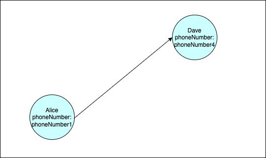
The updates will be applied to ‘B’ labelled edges since it is the next label after the current latest label ‘A’.
Also, we will apply the combined updates across the last two batch update files to ‘B’ labelled edges, leading to the following graph:

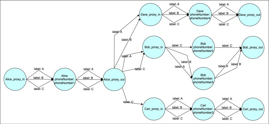
Steps:

• Query the version datastore to fetch the label corresponding to the latest version. In this case, it is ‘A’. The next version will be created with the next label, which is ‘B’. Combined updates across the last two batch update files will be applied to ‘B’ labelled edges.
• To remove ‘Carl’ from this version, remove ‘B’ labelled edge connecting ‘Alice_proxy_out’ to ‘Carl_proxy_in’
  
  • g.V().hasId('Alice_proxy_out').outE('B').as('edge').inV().hasId('Carl_proxy_in').select('edge').drop()
• Add ‘B’ labelled edge connecting ‘Alice_proxy_out’ to ‘Dave_proxy_in’
  
  • g.V('Alice_proxy_out').as('fromV').V('Dave_proxy_in').as('toV').addE('B').from('fromV').to('toV')
• Move ‘B’ labelled edges connected to ‘Bob’ with ‘phoneNumber2’ to ‘Bob’ with ‘phoneNumber5’
  
  • g.V().hasId('Bob_proxy_in').outE('B').as('edge').inV().hasId('Bob').select('edge').drop()
  • g.V().hasId('Bob').outE('B').as('edge').inV().hasId('Bob_proxy_out').select('edge').drop()
  • g.V('Bob_proxy_in').as('fromV').V('Bob_2').as('toV').addE('B').from('fromV').to('toV')
  • g.V('Bob_2').as('fromV').V('Bob_proxy_out').as('toV').addE('B').from('fromV').to('toV')
• Remove ‘B’ labelled edge from ‘Alice_proxy_out’ to ‘Bob_proxy_in’
  
  • g.V().hasId('Alice_proxy_out').outE('B').as('edge').inV().hasId('Bob_proxy_in').select('edge').drop()
• Update version datastore with the following mapping:
  

• Client service can then query version 0 using label ‘C’, version 1 using label ‘A’, and version 2 using label ‘B’, using the following steps:
  
  • Query the version datastore to fetch the edge label corresponding to the required version. E.g: for version 2, the label is ‘B’.
  • Query the graph using the edge label. Sample Gremlin query to get outgoing nodes from ‘Alice’ in version 2: g.V().hasId('Alice_proxy_out').outE('B').inV().outE('B').inV() – returns ‘Dave’

This cycle continues every week. For example:At week 3, when the next batch update file is received, the changes across the last three batch update files are applied to ‘C’ labelled edges, and the version datastore is updated to map label ‘C’ to version 3.
At week 4, when the next batch update file is received, the changes across the last three batch update files are applied to ‘A’ labelled edges, and the version datastore is updated to map label ‘A’ to version 4.

In the end, we will call out a couple of implicit assumptions we made in this blog:

• It was assumed that one update file is received only after the previous one has been fully processed. This should not be an issue, though, since it should be possible for a system to schedule updates sequentially.
• We also assumed that there are no dangling nodes in the graph, that is, nodes that are not connected to any other nodes. If your graph has such nodes, they can’t be queried using the techniques we discussed in this blog.

Also, a connected node can eventually become dangling if all edges connected to it are deleted. At this point, such a node can no longer be queried.
If the application does not need to retain dangling nodes, it is best to delete them. One can run a periodic job that detects such nodes and deletes them using a query like g.V().not(inE()).not(outE()).drop()
Alternatively, one could do so while deleting edges.

• https://arangodb.com/learn/graphs/time-traveling-graph-databases/
• https://arangodb.com/2018/07/time-traveling-with-graph-databases/
• https://medium.com/neo4j/keeping-track-of-graph-changes-using-temporal-versioning-3b0f854536fa

DISCLAIMER: The views expressed in this blog are solely those of the author and do not represent the views of Amazon. The information presented in this blog is for informational and educational purposes only. The author provides no guarantees or warranties regarding the accuracy, completeness, or usefulness of any content.

Users acknowledge that any reliance on material in this blog is at their own risk. Amazon does not endorse any third party products, services, or content linked from this blog. Any links or reference to third party sites or products are provided for convenience only. Amazon is not responsible for the content, products, or practices of any third party site.

The author reserves the right to make changes to this blog and its content at any time without notice. This blog may contain the author's personal opinions, which do not necessarily reflect those of Amazon.